Introduction
Structural MRI is often treated as if it were a ruler for the brain: we talk about hippocampal volume, cortical thickness or white-matter changes as if they were simple, precise measurements. In reality, every number comes from a long processing chain – scanner, reconstruction, segmentation – and each step adds a little variability. Over time, real change in the brain has to be separated from this measurement noise. But how big is that day-to-day wobble in practice?
To get a feel for this, I scanned the same individual twice, three days apart, and processed both scans with FreeSurfer. The logic is simple: anatomy should not change over three days, so any differences in estimated brain volumes and cortical thickness mainly reflect the combined variability of the scanner and the processing pipeline. This is a small N = 1 experiment, but it gives a concrete sense of how stable these widely used morphometric measures really are.
Data and Processing
Both sessions used a 3D T1-weighted MPRAGE on a 3T Siemens Prisma with 1×1×1 mm isotropic voxels, acquired in about 5 minutes using a 64-channel head/neck coil and GRAPPA acceleration (factor 2). This is a standard high-resolution structural protocol that provides good gray–white contrast for surface reconstruction and volumetric segmentation. Both T1 images were converted to NIfTI and processed with FreeSurfer’s recon-all pipeline inside an Ubuntu Linux virtual machine running on my Windows laptop.
Each run of recon-all took roughly three hours and produced the usual collection of outputs: skull-stripped volumes, cortical surfaces, subcortical and cortical segmentations, and regional statistics files. I used FreeView for visual quality control of the segmentations and surfaces, then exported summary measures (global volumes, subcortical volumes, and cortical thickness/area/volume per region) into tidy .tsv files for analysis in R. The goal was to look systematically at how close Session 1 and Session 2 estimates are across the whole brain.
What FreeSurfer actually does to the brain image
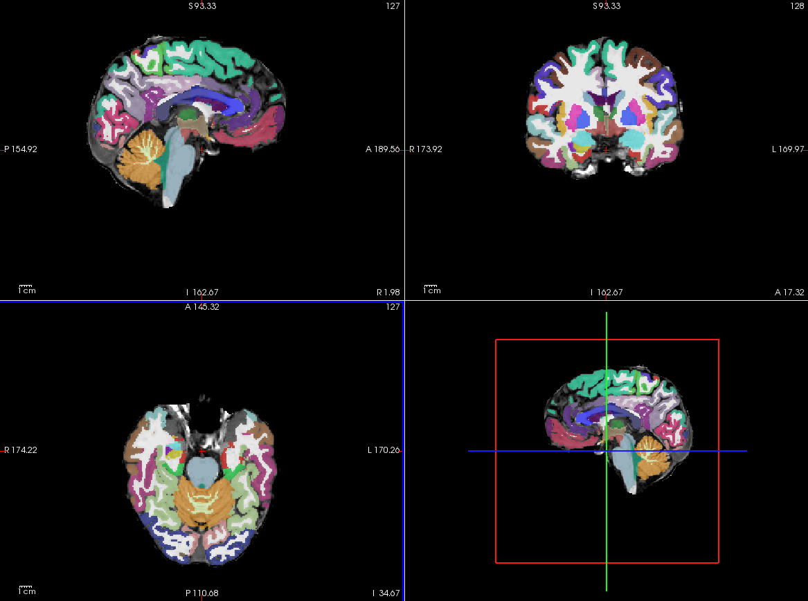
This view shows the final parcellation that most people think of as “the FreeSurfer output”: cortical regions from the Desikan–Killiany atlas overlaid on the T1 image, together with subcortical structures and cerebellum. Each colour corresponds to a label in aparc+aseg.mgz, which is what later gets turned into regional volume and thickness estimates. The three orthogonal slices and the 3D inset make it easy to see that sulci and gyri are generally well followed, with only minor imperfections along some boundaries.

Here only the subcortical and cerebellar labels from aseg.mgz are shown. Deep nuclei such as thalamus, caudate, putamen, pallidum, hippocampus and amygdala are clearly delineated, as are ventricles and brainstem. These labels are the source of the “aseg volume” statistics that I compare across sessions in the plots below.
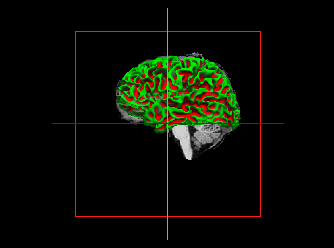
This figure shows the reconstructed white-matter surface (green) overlaid on the T1-weighted image. The mesh follows the grey–white boundary throughout the cortex; in most areas the fit is tight, with occasional local mismatches around difficult regions such as temporal poles and medial frontal cortex. This surface provides one of the two boundaries used to compute cortical thickness.

Here the cortex has been “inflated” to smooth out sulci, and vertex-wise cortical thickness is overlaid as a heatmap. Gyri and sulci are still recognisable, but the inflation makes it easier to see spatial patterns in thickness without deep folds occluding the view. This is mainly a qualitative QC tool in this post, but in group studies these maps are often used for vertex-wise statistics.
Results
Subcortical and global volumes
Across most global and subcortical measures, Session 1 and Session 2 volumes agreed within a few percent. The largest structures – cortical grey matter, cerebral white matter, cerebellar cortex and total intracranial volume – differed by well under 2% between scans, which is reassuring given that these are the workhorses in many morphometry papers.
A few non-neuroanatomical aseg labels (for example, vessel and SurfaceHoles) showed very large percentage differences despite tiny absolute volumes. These labels are essentially bookkeeping regions used by the segmentation algorithm; because their true volume is close to zero, even small absolute differences translate into very large relative changes. In this context they are better treated as QC indicators of how the algorithm behaved than as meaningful anatomical measurements, and I did not interpret them further.
Among the classical subcortical nuclei, the pallidum, putamen and amygdala showed somewhat higher variability than, say, the thalamus or caudate. That pattern is in line with previous reports that their boundaries are harder to define reliably on standard-resolution T1-weighted scans, so their test–retest stability is typically a bit worse. In contrast, most other subcortical and global cortical volumes differed by only a few percent, suggesting that for large structures, FreeSurfer plus a modern 3T scanner is reasonably stable over a timescale of days.
The complementary plots using absolute percent differences (|100 × (ses-02 – ses-01) / ses-01|) make this pattern clear: the bulk of regions cluster at low single-digit differences, with a tail of more variable labels that are either very small (e.g. vessels, surface holes) or anatomically challenging.


Cortical parcellations – Destrieux atlas (aparc.a2009s)
The Destrieux atlas divides the cortex into a much larger number of relatively fine‐grained gyri and sulci, so here I looked at test–retest differences in surface area, thickness, and volume for each parcel and hemisphere. The heatmaps show that most regions cluster fairly close to zero, with the bulk of percent differences in the low single digits for both hemispheres. Thickness is the most stable metric: for the overwhelming majority of parcels, Session 1 and Session 2 estimates differ by only a couple of percent
Area and volume show more spread, with a tail of parcels where the test–retest difference reaches several tens of percent. These high-variance labels tend to be anatomically tricky regions – thin ribbons along deep sulci, orbitofrontal cortex, and medial temporal structures such as the parahippocampal and entorhinal regions – where even small shifts in surface placement or partial-volume effects can change the measured area or volume quite a lot. The hemisphere-summary panels make this pattern clearer: distributions for left and right hemispheres overlap almost perfectly and are centered near zero, but with a slightly wider spread for area and volume than for thickness. Overall, the Destrieux parcellation behaves reasonably well at the group level, but individual parcels – especially small or complex ones – can show sizeable test–retest variability.

Cortical parcellations – DKT atlas (aparc.DKTatlas)
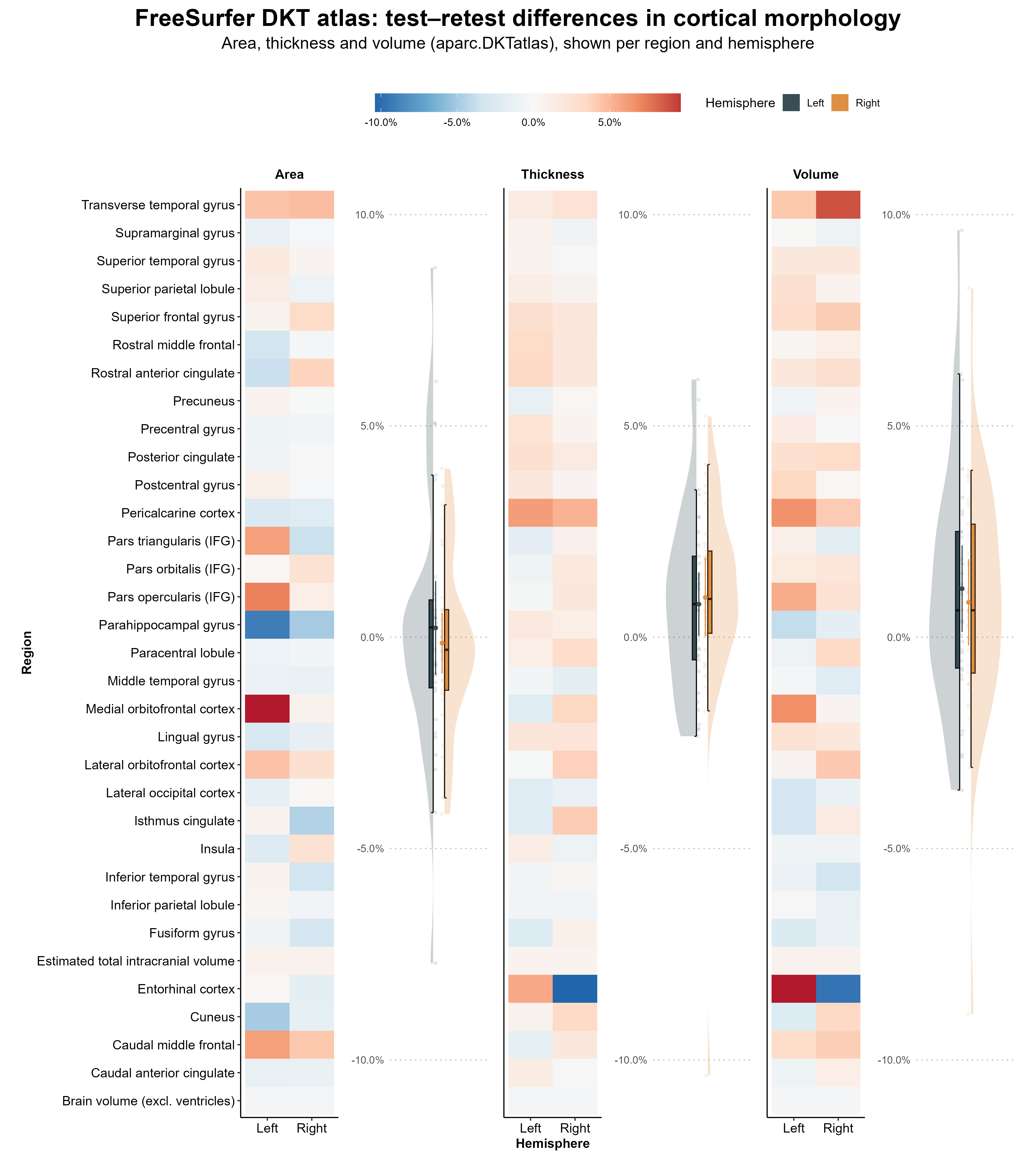
The DKT atlas uses fewer and coarser cortical regions, so each parcel covers a larger stretch of cortex. Under the same metric (percent difference between Session 1 and Session 2), the DKT results look noticeably more conservative than the Destrieux atlas. Across most regions, area and volume estimates stay within roughly ±5–10%, and thickness differences are generally smaller still, clustering tightly around zero for both hemispheres.
A few parcels still stand out with higher variability – again mainly in border zones such as orbitofrontal, entorhinal and medial temporal areas – but the overall color range is much more muted than in the fine-grained Destrieux plots. The hemisphere-summary panels show overlapping distributions with very similar medians for left and right, and no obvious systematic bias towards one hemisphere. Taken together, this suggests a familiar trade-off: coarse DKT regions yield more stable test–retest estimates, while the more detailed Destrieux parcellation offers finer spatial resolution at the cost of increased variability in some small and anatomically challenging parcels.
Take-home message
Over just three days, most FreeSurfer measures in this N = 1 test–retest dataset were remarkably stable: global volumes (total cortical and subcortical grey matter, cerebral white matter, cerebellum, ventricles) and the majority of cortical regions differed by only a few percent between sessions. Cortical thickness was especially consistent, with very small test–retest differences across both the DKT and Destrieux atlases. In contrast, a minority of labels showed much larger percentage changes – either because they are tiny, algorithmic “bookkeeping” regions (for example, vessel, SurfaceHoles) where even a few voxels make a big relative difference, or because the underlying anatomy is harder to segment reliably (such as pallidum, putamen, amygdala and certain orbitofrontal or medial temporal parcels). These outliers are probably better viewed as QC-sensitive regions than as precise longitudinal biomarkers, whereas large global structures and most cortical parcels appear reasonably robust over short timescales on a modern 3T scanner.